
For example, the voltage, current and conductance electrical magnitudes can be used as analogues of fluid pressure, flow rate and tube diameter. More specifically, in traditional analogue computing, the values ??resulting from the calculation obey the same mathematical laws as the physical quantities in the primary system. Thus, computational quantities are proportional to the modelled quantities. [2]
The analogue computer is based on circuits that can calculate or process measurements, quantities, or continuous functions in time. Among such analogue circuits, those based on operational amplifiers can be used to implement mathematical functions and are also useful in many applications due to their technical and functional characteristics.
When we touch the words "computer" or "computing", we usually associate them with digital systems. It currently makes sense since most computer systems operate based on binary and discrete structures. At first, analogue computing was eventually forgotten, given the great advantage of digital techniques in various aspects.
However, before digital computing became commonplace, analogue computing was widely used to calculate and solve well-defined functions such as sum, subtraction, multiplication, division, absolute value, maximum/minimum, RMS, peak, square roots quadrature, derivatives, exponentials and integrals. [1]
It was found over time that analogue computing still had its place in academia and in specific scientific research, where its characteristics still had room to contribute since it can avoid the limitations of digital computing. [2]
Recently, research on non-traditional computing (also unconventional or exotic) is taking place in materials physics, chemistry, and more "exotic" branches such as biology and life sciences. [3]
These aspects make it very interesting to revisit the fundamentals and origins of analogue computing and its achievements. Remember that the slide rule is an example of an analogue computer, which participated in numerous aerospace engineering projects and even the Apollo 11 mission to land man on the Moon. On the Newton C. Braga Institute website, on analogue computing [4], the reader can find much information on this topic. Figure 1 shows an analogue computer.

2. History Of Analogue Computing From The Electronic Age
Analogue electronic computers became viable after the invention of the DC operational amplifier. Scientists from the 1930s Bell Telephone Laboratories (BTL) developed the feedback-stabilised DC-coupled amplifier that is the basis of the operational amplifier. Soon engineers in the 1940s saw applications of electronic analogue computing for military, research and science, giving birth to the GPAC - General Purpose Analogue Computer, also called "Gypsy", completed in 1949. Based on the design of the BTL operational amplifier, work on this computational platform was handled at Columbia University in the 1940s. In particular, this research showed how analogue computing could be applied to the simulation of dynamical systems and the solution of non-linear equations.[2]
3. How An Analogue Computer Based On Operational Amplifiers Works
An analogue computer consists of modular circuits capable of individually performing operations such as adding, scaling, integrating or multiplying voltages. These sets are connected to function generator modules. Such circuits are composed of operational amplifiers arranged in tens or hundreds of modules, forming a large analogue computer.
To solve a given problem where physical quantities vary over time, we can represent such a problem through differential equations. The solution of these equations is accomplished through the proper interconnection of analogue circuit modules with their inputs and outputs, incorporating scaling, feedback and definition of initial conditions as necessary with voltages representing the physical model variables [5].
Thus, simple or simultaneous equations can be solved in engineering and scientific calculation, modelling and simulation. The interconnection and definition of required initial coefficients and conditions are typically achieved through a patch panel and potentiometers. As input, function generators are used. As output, oscilloscopes or a data recorder are used.
When using the analogue computer for research or development, the designer can immediately observe the effect by modifying the voltages corresponding to the mathematical parameters through the respective potentiometers or switches. In simulations, the analogue computer outputs can be used as input voltages for another electronic system intended to be controlled. [5]
3.1 Arithmetic And Mathematical Function Operators
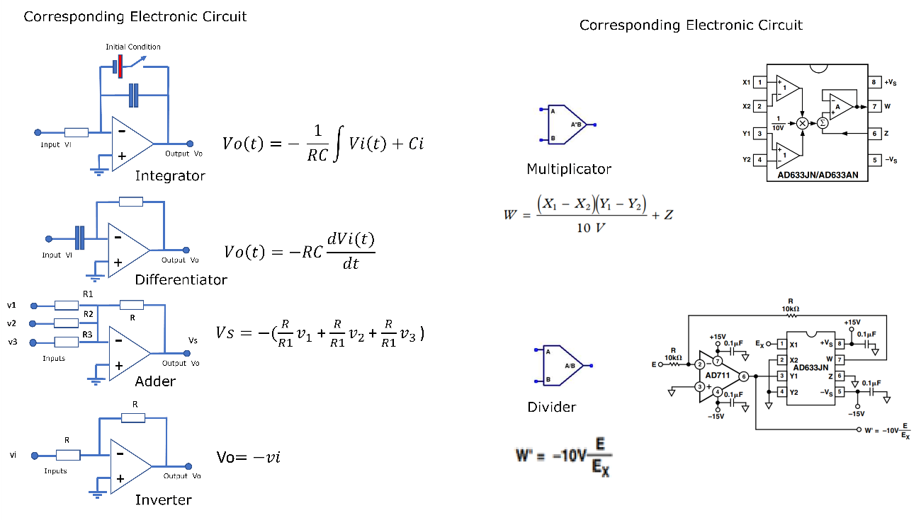
The basic building blocks of mathematical operators in an analogue computer are adders, inverters, multipliers, divisors, integrators and differentiators. Refer to Figure 2.

When receiving inputs, each block processes such signals to generate output signals corresponding to the mathematical operation. These signals, in the case, voltages, should represent with their values ??the quantities previously identified and belonging to the physical model. In Figure 3, we have the electronic equivalents to the blocks of an analogue computer.
4. Example Of An Analogue Computer And Its Application In A Dynamic System
The behaviour of time-varying physical, chemical or biological phenomena can be described through mathematical models that link the present state to past states, represented by dynamical systems.
When designing mechanic and mechatronic systems and considering the system's degrees of freedom, we have to contemplate the dynamic behaviour so that the system executes its movements with the appropriate force, torque, speed, and position to perform them quickly and accurately. Vibrations, positioning errors, loss of force due to speed, among other factors, are parameters considered in the design of such systems.
As an application example of an electronic analogue computer, we will exemplify the simulation of a mechanical system representing 1/4 of a car suspension illustrated in Figure 3. The objective is to obtain the best response of the physical system when subjected to variations that simulate conditions of the terrain or track.

Considering the best conditions of this mechanical system, we must avoid unwanted oscillations or even resonance effects that can make the operation unstable with catastrophic consequences. Conversely, a too slow system to respond to terrain variations can be equally detrimental to performance. Therefore, for the system to be designed satisfactorily, a mathematical model that represents this system must be elaborated so that, through simulations, the parametric coefficients can be adjusted.
At this point, digital or analogue computational simulation methods are applied. In our example, the system will be simulated using analogue computation [8].
First, the system is modelled by analysing its components and the physical behaviour of each one. Then, when composing the system, the physical models are represented by differential equations, which respond with corresponding output signals when submitted to input functions. In our example, the equations describing the physical model are in Figures 4a and 4b.


We can assemble a system of equations used to "program" our analogue computer from these models, as shown in Figure 5.

Now, through the configurable blocks, we connect them to represent the set of equations as shown in Figure 6.

Observing the properly structured analogue computer at the Zr input, we subjected the system to oscillations similar to those found in a road, a track, dirt, etc. We assume that the suspension is subjected to a sudden variation through a step-like impulse, representing, for example, an elevation, a stone or a hole. To control and adjust the system parameters so that the response is as fast and smooth as possible, we change the coefficients A, B, C, D or E, related to the physical quantities involved (Force, Velocity, Viscosity, Elastic Constants etc.). The response to this step can be seen and recorded and the parameters adjusted by equivalence between the coefficient and the voltage to be placed on the inputs.
Analogue computing will simulate the mechanical system and its responses to simulated impacts, generating electrical signals equivalent to the magnitudes. We can change the simulation responses until we get the desired response parameters by changing and adjusting the coefficients A, B, C, D, E. As an example, the Zr step simulates an impact generated by the road or track. The mechanical responses to this impact are represented by the Zs curves shown in Figure 7. In practical terms, the suspension can oscillate in an under-damped way, generating instability in the vehicle, or in a critically damped way, dampening the impact quickly and efficiently, or over-damped, where the impact is applied, but the system is slower to recover from the excitation in Zr, which can also destabilize the vehicle. Note that the analogue computer responds electrically, generating signals that correspond to the quantities tested.

5. Merging Analogue Computing, Signal Processing and Digital Computing
Today's computers, used to control systems and signal computation, are based on high-performance systems with DSP (Digital Signal Processors) type processors, which are extremely fast. Its architecture was designed for processing signals at increasingly higher frequencies. One of the current examples is digital oscilloscopes, which are based on DSPs. When processing signals, they need to convert analogue inputs into digital (A/D) through techniques that preserve the characteristics of the analogue signal after the process. Once converted into data, the processor applies the desired mathematical algorithms, obtaining the result of this processing in its output and storing it in memory. The next step is to perform the digital to analogue (D/A) conversion or use the digitized data for math operations, plotting signals on displays, etc., with accuracy. Thanks to these characteristics, analogue computers lost relevance since analogue variables need to be very well controlled to obtain accurate results and the enormous benefits that DSPs have brought into many electronic devices and instruments. Thus, analogue computers were restricted to specific scientific applications in universities.
Analogue Computing Perspectives
With technological advances in analogue circuits, the feasibility of composing hybrid systems between analogue and digital computers improves since a good part of the problems of analogue computers related to the control of variables and errors are being solved through integration and new technologies in operational amplifiers. Thus, the benefits of analogue computing to work continuously over time complement the steps used by digital systems, processing signals that will later be digitized and processed more simply by DSPs. Therefore, when working together, the capacity and performance of hybrid systems are very promising. [9][10]
References
[1] Scheber Bill Analog computation, Part 1: What and why jan 14, 2019 – Article https://www.analogictips.com 28/05/2021
[2] MacLennan Bruce J. A Review of Analog Computing Technical Report UT-CS-07-601 * Department of Electrical Engineering & Computer Science University of Tennessee, Knoxville September 13, 2007
[3] Köppel S. Ulmann B, Heimann L. Killat D, About using analog computers in today’s largest computational challenges GmbH, Am Stadtpark 3, 12167 Berlin, Germany Microelectronics Department, Brandenburg University of Technology
[4] https://www.newtoncbraga.com.br/index.php/computacao-analogica/16420-computacao-analogica-licao-1-os-computadores-analogicos-cur6001.html - 28/05/2021
[6] AD 633 Low-Cost Analog Multiplier Analog Devices datasheet Analog Devices, Inc., 2002
[7] Kluever, Craig A. Sistemas dinâmicos: Modelagem, simulação e controle. São Paulo: LTC, 2017.
[8] Introduction to analog computing - Article https://www.elettroamici.org/en/ 31/05/2021
[9] Huang, Yipeng Hybrid Analog-Digital Co-Processing for Scientific Computation –Rutgers University 08/05/2021
[10] Crane, L Back to analog computing: merging analog and digital computing on a single chip Article COLUMBIA UNIVERSITY IN THE CITY OF NEW YORK Electrical Engineering December 04, 2016


