
Note: Article published in Saber Eletrônica Magazine, issue 194, 1989. ART3577S ART5271
A Dip Meter is nothing more than a high-frequency oscillator with interchangeable coils and special features. Operating freely, it generates a signal of known frequency, thus serving to determine points on the receiver tuning scale. However, when its oscillating coil approaches any resonant circuit (a coil and a capacitor), an important phenomenon occurs, When the circuit's frequency matches that of the nearby LC set, a change in internal conditions occurs that alters the field-effect transistor's drain current, and this can be easily visualized on an instrument.
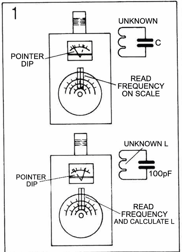
To do this, simply bring the device close to the unknown LC circuit and adjust the internal oscillator frequency until a change in current (as detected by the instrument) is observed. At this point, we read its resonant frequency directly from the scale (Figure 1).
To determine the inductance of a coil, simply proceed in the same way, connecting a capacitor of known value in parallel with it. With the resonant frequency value, we can easily calculate the inductance, as we will explain. The circuit operates with a voltage of 9V, which can be supplied by a small battery, making it completely portable.
We will provide instructions for winding three coils to cover frequencies between 1.2 and 25MHz, but there is nothing to prevent additional coils from extending this range to 100MHz, if some precautions are taken to avoid dead spots on the scales or instability. In addition to the uses suggested in the introduction, the Dip meter also serves as an excellent signal generator for calibrating receivers.
THE CIRCUIT
In the "old days" of vacuum tubes, a very popular instrument among experts was the "Grid-dip Meter."
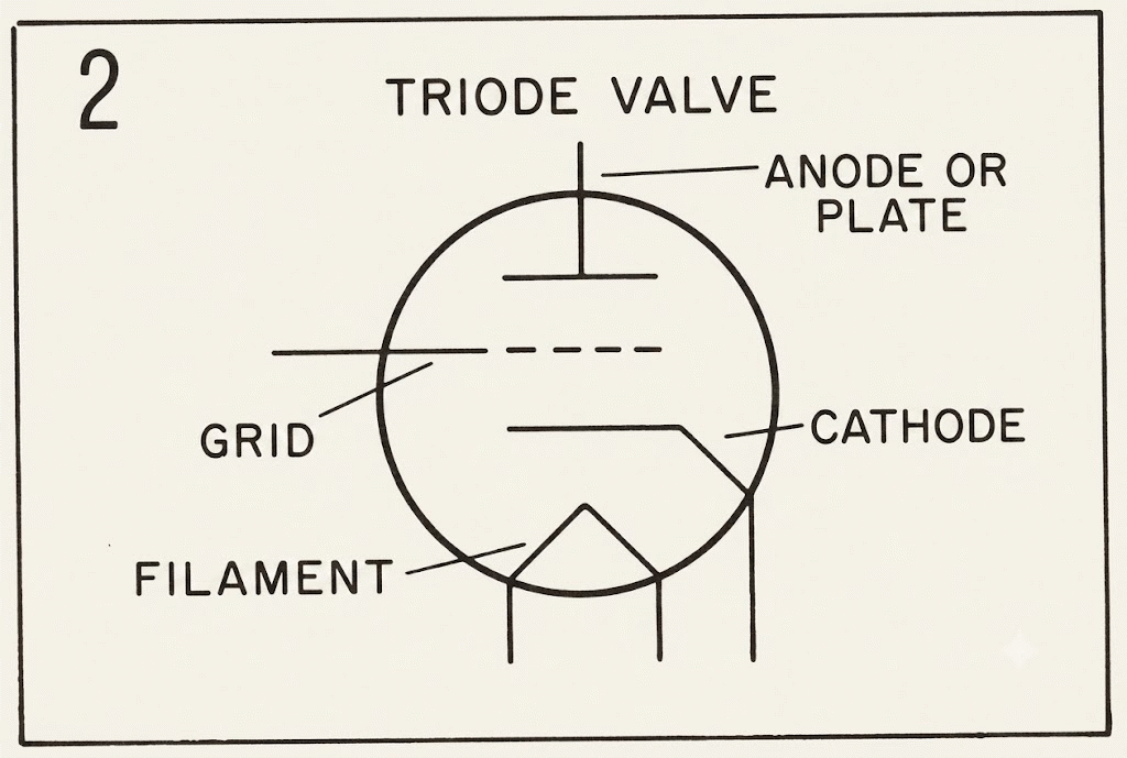
This name derives from the fact that we have a triode tube, in which one of the elements is the grid, and which was connected in such a way as to operate as a high-frequency oscillator (Figure 2). When this circuit was brought close to an LC resonant system, with a coincident frequency, a drop or "dip" occurred in the grid current that could be detected by a sensitive instrument.
In the modern version, we replaced the triode tube with a field-effect transistor (FET), and instead of having a variation in the "gate" current, since in an FET its high impedance prevents this from occurring, we have a variation in the drain current (D). Therefore, when we bring the coil of the dip meter oscillator circuit closer to an LC resonant circuit, there is a sharp drop in the drain current, or a "dip" in the indicator needle of the instrument used.
If the instrument is equipped with a variable capacitor and an appropriate set of coils that allows it to cover a wide frequency range, it becomes an extremely useful tool for determining resonant frequencies and, immediately, for calculating small inductances. The circuit we describe does just that: the BF245 field-effect transistor is connected as a Hartley oscillator, where LX and CV determine the operating frequency. Feedback comes through C2, and gate bias is provided by resistor R1.
To detect drain current variations, we connect a 0-200 µA microammeter (approximately) along with an adjustment potentiometer, which allows the pointer to easily position itself at the center of the scale during normal operation. By adjusting CV, we can reach the point where the frequencies between the dip meter and the LC circuit under analysis coincide. At this point, the drain current drops, causing the voltage across M1 to rise, resulting in a sharp deflection of the instrument's pointer. This deflection occurs in the sense that there is a drop in the indicated voltage, since the bridge is balanced with a positive value on the P1 cursor side. We then experience a true "dip" of the instrument's needle when resonance is encountered.
Operation above 30MHz encounter two types of problems that require skill from the assembler: the first concerns the coils, which must have few turns with minimal parasitic capacitance. The second concerns the value of CV1, which must eventually be reduced. Thus, to extend the range to 100MHz, for example, we must also change the lower operating limit, which should increase to around 5MHz.
ASSEMBLY
Figure 3 shows the complete diagram of the device.
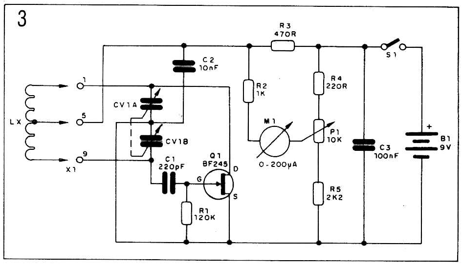
Note that this is a very simple circuit, as few components are used. However, since this is a device that operates at high frequencies, some care with the arrangement of the parts is important to avoid parasitic capacitance and instability. Figure 4 shows the printed circuit board, which is quite simple.
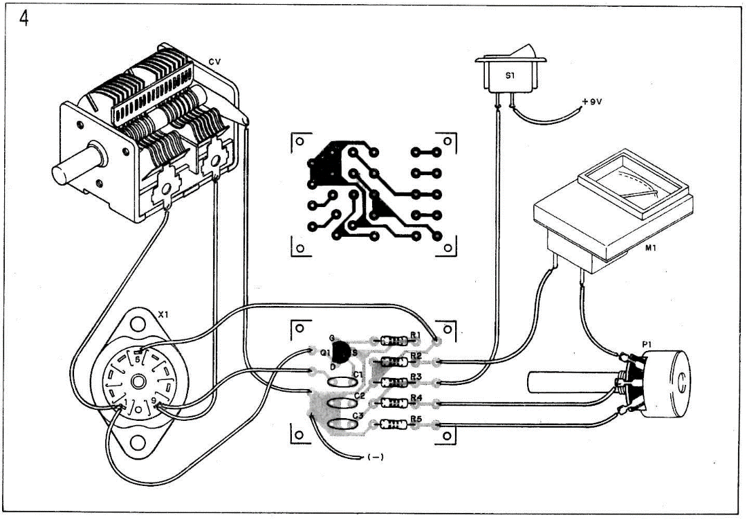
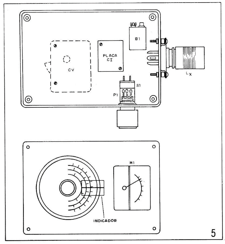
Figure 5 shows the internal layout of the assembly, with the components arranged in a 12 x 8 x 5cm Patola box.
The variable is a two-section type, salvaged from a disused tube radio, and its value is not critical, as this is the function we use to calibrate the scale. Variables with maximum capacitances in the range of 190 to 300 pF can be used. In fact, you should not worry about the exact value of this component's extreme capacitances, as we will teach you how to calibrate the device without considering this. Simply use the variable of the type used in old medium-wave radios, with two sections and a thin shaft for attaching the button, and the problem is solved!
The instrument is a microammeter of the type used as a VU in stereos. Its value is not critical, with a full-scale range between 100 and 300 µA. Even a 0-1mA milliammeter can be used by replacing P1 with a 2k2 potentiometer.
This potentiometer can incorporate a master switch, as in the prototype, thus facilitating the device's use. The resistors are 1/8W with 10% tolerance, and the capacitors are all high-quality ceramic. For Q1, we can use a BF245 or an MPF102. In the case of the MPF102, however, the terminal layout is different, which must be considered when placing it on the board.
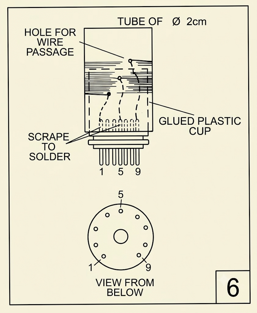
For a variable capacitor with approximately 210pF of maximum capacitance, we provide coils with the frequency ranges covered, but since tolerances may exist, the values are approximate. The exact calibration will be explained later. All coils (3) are wound on 2cm diameter cardboard tubes with lengths varying between 2 and 4cm (depending on the number of turns).
The DIP meter is connected using a Noval socket and corresponding 9-pin base, the type used for tubes. In figure 6 we show details of the construction of one of these coils.
The following table lists the number of turns and the frequency range covered by the corresponding coil. Note that the coils have a center tap and are wound with 28AWG enameled wire.
Range (MHz) = Turns
0,5 to 1,8 = 1,5 to 5
4 to 25 = 45 + 45
22 + 22 = 12 + 12
To reach 40MHz, the coil can be 7+7 turns; however, depending on the variable, dead spots may occur in the tuning, that is, points without oscillation. The variable should have a maximum capacitance of around 80pF for this case. The same applies to a frequency of 80MHz, where we have approximately 4+4 turns. To construct the coil, the enameled wire can be held in place using glue or even candle wax. To connect the battery, we use a special connector. This can be secured with a clamp.
To the variable, we attach a knob that allows for a triple scale (or quadruple, if you wind four coils). This knob is the type found in transistor radios, where a piece of transparent acrylic with a red line serves as a reference for adjusting the desired frequencies.
CALIBRATION
This is the most delicate step in the assembly process, requiring the assembler to have a medium- or short-wave receiver that covers the dipmeter's operating range or a frequency counter. We will use the receiver to perform the procedure, as the frequency counter allows for immediate operation.
Start by placing the coil that covers approximately 0.5 to 1.8 MHz (depending on your variable and even small variations in component values, significant differences may occur within this range, but you will easily determine this). Turn on your receiver to the medium-wave band and close the dip meter is variable. Place the receiver about 30 cm away from the dip meter and rotate the tuning dial until you pick up the oscillator signal in the form of a "whisper" or slight hiss. It may also be a whistle if the frequency coincides with a local station.
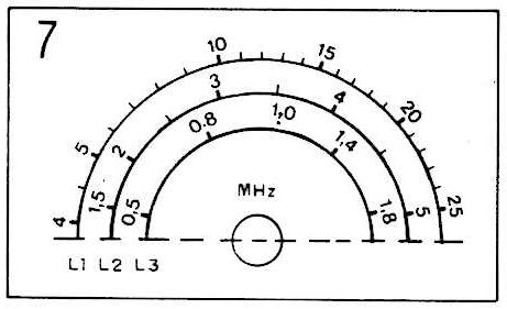
At this point, you have the first frequency reference for your scale. If nothing is picked up, leave the receiver variable at the lowest frequency in the medium-wave band (530 kHz) and gradually open the dip meter variable until the signal is picked up. You then have the new reference for your scale. Note that it's a good idea to know exactly what the rotation angle of your variable is beforehand and have a piece of paper ready to record the values (Figure 7).
When locating the DIP meter signal, it's important to be careful not to mark the frequency of a harmonic oscillation, that is, a multiple of the original frequency, which can result in an incorrect scale. The fundamental signal is the strongest, captured throughout the entire range of the DIP meter, and this can produce a variety of signals. From the first point found on the scale, we can gradually find others, using the radio as a reference.
Thus, in the case of the medium-wave band, simply tune the radio to 800 kHz and adjust the DIP meter until the signal is captured. We then mark 0.8 on the corresponding scale.
We do this with frequencies of 1, 1.3, and 1.6MHz, or as far as the coil reaches, since, as we have seen, variations can occur depending on the components used. The important thing for the assembler is that, once this calibration is done, it will be valid for their coil, and they will no longer need a radio to know the frequency at which the circuit is operating.
If we finish the receiver band without having all the DIP switches open, we must move on to the other band to find new points. We proceed in the same way with the other coils, always using the frequencies tuned to the receiver as a reference, in the medium and shortwave bands. Hence, the need for a receiver with as many bands as possible and properly calibrated. To determine if your receiver is truly calibrated, you can use known stations that are easily tuned.
USE
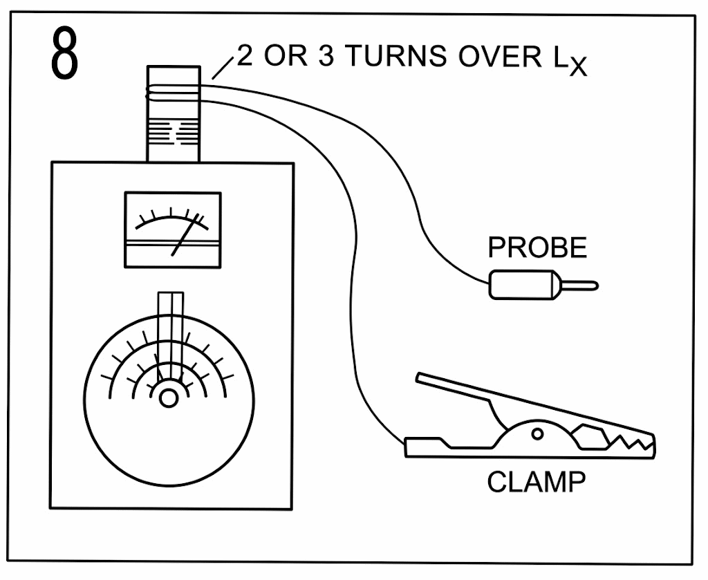
As a signal generator, simply adjust the frequency on the scale with the coil that covers the desired band, and then bring the DIP Meter closer to the device where you want to inject. A coupling link can be improvised, as shown in Figure 8, for less sensitive circuits.
To determine the inductance of a coil or the resonance frequency of an LC circuit, proceed as follows: connect a 100pF ceramic capacitor in parallel with the coil if you want to know its inductance; for an LC circuit, leave it as is. Bring the dipmeter close to the coil and adjust the potentiometer so that the instrument reads approximately mid-scale.
Place a coil on the dipmeter according to the frequency at which resonance is expected. Continue turning the variable until you notice a sudden movement of the instrument needle (a drop). At this point, simply read the resonance frequency. For the coil, use the following formula to calculate the inductance:
where: C is the capacitance, in farads (100pF = 100 x 10-12F)
F is the frequency read, in Hertz
L is the inductance, in Henry (H)
Note: If the pointer tends to deflect in the opposite direction to the expected, reverse the connections.
LIST OF MATERIALS
Q1 BF245 field-effect transistor (Philips)
M1 0-200μA - microammeter
B1 - 9V battery
Lx - coils - see text
CV - 2-section variable 290+290pF
-see text
C1 - 220pF ceramic capacitor
C2 - 10nF ceramic capacitor
C3 - 100nF ceramic capacitor
R1 - 120k resistor (brown, red, yellow)
R2 - 1k resistor (brown, black, red)
R3 - 470ohm resistor (yellow, violet, brown)
R4 - 220ohm resistor (red, red, brown)
R5 - 2k2 resistor (red, red, red)
P1- 10k potentiometer with switch
S1 - single-ended switch (coupled to P1)
Miscellaneous: printed circuit board, mounting box (Patola) Ref. 15), connector for 9V battery, Noval socket for valves, 9-pin plug, cardboard tubes for the coils, 28AWG enameled wire, knob for the potentiometer, knob for the variable, solder, etc.


